Interferómetro - o - Sensor de frente de onda

La tecnología evoluciona, al igual que los sensores de frente de onda. Una de las mejoras más notables ha sido la densidad de muestreo del frente de onda. Algunos ejemplos son los sensores HASO LIFT de Imagine Optics y el sensor QWLSI de Phasics. Las técnicas para lograr esta densidad de muestreo mejorada difieren.

La técnica LIFT, también conocida como técnica de plano focal linealizado, es una nueva versión del método utilizado antiguamente para mantener el enfoque en reproductores de DVD y CD. Se añadía una lente cilíndrica para proporcionar astigmatismo adicional (en el eje) en la trayectoria del haz reflejado. Cuando el disco estaba enfocado, el detector cuadrante mostraba la misma señal en las dos celdas diametralmente opuestas. Fuera de foco, había una diferencia, incluido el signo, que podía utilizarse como retroalimentación.

Con el mismo espíritu, la técnica LIFT añade astigmatismo en el eje, pero muestrea el punto focal con una resolución mucho mayor y, de este modo, puede resolver muchos más términos que una simple curvatura del frente de onda.

El enfoque QWLSI fásico, por su parte, emplea la interferencia para crear un patrón de franjas bidimensional. Mediante métodos de franjas de Fourier, se extraen dos gradientes de frente de onda y se integran para obtener el frente de onda.

Interferometría, precisión y resolución

Aunque parezca que LIFT y QWLSI no tienen nada en común, sí lo tienen. Ninguno de ellos puede medir la desviación en términos absolutos en el sistema de espejos deformables que se esboza a continuación. ¿Importa esto? Bueno, depende de lo que se quiera conseguir. Lo que hará bastante bien es medir la forma del espejo dada la señal, lo que en muchos casos es bastante bueno. Para el ejemplo del esquema, en el que no podemos ver todo el espejo, no tenemos suerte.

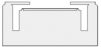
El término pistón, tan a menudo ignorado, no es producto de la imaginación de nadie. En un interferómetro bien diseñado, puede ser una baza fiable para todo tipo de aplicaciones. Este espejo deformable es quizá esotérico, pero la calibración de un modulador de fase de cristal líquido puede hacer buen uso de él. El caso óptico es bastante similar. La abertura transparente no conecta con una fase fija, y los campos de franjas devalúan la eficacia de utilizar el valor integrado de un gradiente de fase.

Precisión y grados de libertad abiertos

En primer lugar, ¿qué quiero decir con grados de libertad abiertos? Con esto me refiero a los grados de libertad que contribuyen directamente al error de medición. Se pueden calibrar, y normalmente se hace, pero se trata de una sensibilidad lineal. Un ejemplo arquetípico de esto es el desplazamiento de las microlentes en un conjunto de microlentes que, a menos que se calibren, hacen que los sensores Shack-Hartmann sean prácticamente inútiles para realizar mediciones precisas del frente de onda. ¿Están abiertas las sensibilidades de píxel de las cámaras? Para el sensor Shack-Hartmann, las sensibilidades lineales de los detectores parecen abiertas, ya que remodelan individualmente las intensidades registradas, pero bajo el supuesto de que las sensibilidades permanecen lineales y constantes, desaparecen en la calibración ya presente de los centros de los puntos.

¿Son necesariamente precisos los interferómetros? No, obviamente no. Hay muchos factores que contribuyen al error total. Sin embargo, en comparación con la mayoría de las soluciones de detección de frente de onda, como diseñadores de sistemas ópticos, podemos tener cierto nivel de control. Como en Senslogic desarrollamos nuestro propio sensor Shack-Hartmann, somos conscientes del valor de calibrar estos dispositivos y del esfuerzo que supone. Dicho esto, cuando se trata de la máxima precisión, nada supera a la metrología cuya exactitud puede atribuirse a un único elemento de precisión.

El ejemplo perfecto es el interferómetro de cambio de fase, o quizá debería haber escrito, a interferómetro de cambio de fase para enfatizar que el cambio de fase es algo que aumenta algún interferómetro específico.

Cambio de fase

Repasemos brevemente el método de desplazamiento de fase y lo que tiene de especial. Prácticamente cualquier configuración interferométrica puede aumentarse mediante el desplazamiento de fase, lo que significa que uno de los dos caminos que puede tomar la luz añade una distancia adicional y bien conocida de sub-longitud de onda con el fin de convertir el análisis de franjas en una simple ecuación para la fase relativa entre los caminos.

El desplazamiento de fase no es en absoluto una tecnología nueva, y en la literatura anterior se encuentran métodos bastante elaborados que implican muchos pasos de fase con el fin de superar las deficiencias de la tecnología predominante disponible en ese momento. Sin embargo, el paso de fase de 90°, introducido desde el principio, ofrece tanta cancelación de errores incorporada que, durante al menos dos décadas, no hubo razón para utilizar otra cosa para analizar una configuración de interferencia de dos haces.

La expresión resultante para la fase,

donde el índice denota el número de pasos de 90° que hemos hecho con nuestro actuador. A y B son las amplitudes reales de los dos haces interferentes, reales porque hemos trasladado la diferencia de fase entre ellos a la fase. Aún más importante es observar que, cuando las intensidades se registran en una cámara, cada píxel nos da uno de los pares de expresiones anteriores para resolver, donde sólo tenemos que dividir,

La expresión anterior está ahora libre tanto de A como de B. Esto es en realidad un problema mayor que puede ser inmediatamente obvio porque tanto A como B dependen de la sensibilidad de los píxeles de la cámara que resulta que los registra en la posición dada, y ahora han desaparecido. Lo que tampoco mencionamos es que cada una de las intensidades puede haber sido grabada en un laboratorio donde hay una fuente de luz de fondo. Esta contribución desapareció en la diferencia entre intensidades tanto en el numerador como en el denominador.

El desfase de 90° se aplica a veces como una medición 4+1 en la que se mide el desfase (aparentemente) redundante de 360&\deg;. Por rudimentario que parezca, el enfoque 4+1 suprime las no linealidades de segundo e incluso tercer orden del detector y errores de escala del actuador. El módulo PSI en WaveMe ofrece tanto el método de las 4 imágenes como el de las (4+1) imágenes, que si no para otra cosa, pueden servir para comprobar que las suposiciones que podamos tener respecto a nuestra configuración son correctas.

Con el cambio de fase, lo primero que necesitamos es asegurarnos de que las diferencias entre las intensidades capturadas sólo reflejan el efecto de nuestro actuador, y como las imágenes se graban en momentos diferentes, cualquier variación temporal aparecerá como un error. Existen métodos que capturan las cuatro fases simultáneamente, pero esto requiere una cámara bastante diferente y el análisis de errores también tendrá un aspecto bastante diferente. James C. Wyant es un defensor muy respetado de este enfoque.

Resumen

Con esta charla técnica, quería aclarar algunos aspectos que hay que tener en cuenta a la hora de elegir entre utilizar un sensor Shack-Hartmann o un interferómetro. Si elige el primero, existen productos de alta resolución en el mercado. Si la resolución no es lo que buscas, no hay mucho que puedas hacer, salvo buscar otra solución. Lo mismo ocurre si necesita el término pistón, o la media de la diferencia de longitud de trayectoria. Tu elección es entonces el interferómetro de desplazamiento de fase. Si no estás contento con la resolución, elige otra cámara. Usted tiene el control. Esto no cambia nada en la aplicación. No hay nueva calibración. Sólo para poner un ejemplo de mi pasado, en el que utilicé lo que había en la mesa en ese momento, que era una cámara pensada para vídeo (no es que sea una diferencia tan grande), pero la cuestión es que, con tanta compensación incorporada, no tienes que preocuparte mucho más allá de tu propia configuración óptica.