


Designing new optical systems from the ground up can be an intimidating task, especially if the system we are trying to make is one that we must get right before anything can be built, because the critical components simply do not yet exist. It’s merely a figment of our imagination, and it is actually part of our task to define it. Similar situations will arise when we explore different designs and want to learn how things actually work before taking on the task of actually building it.
So let’s picture this. You need to find the requirements for a system that we’ve never studied before and if there is a scientific paper that maybe is related to what we need, are we even going to find it? It’s not uncommon that we reinvent the wheel. Dirac reinvented the Clifford algebra when he derived the quantum equations for the electron, so obviously, this happens to the best of us. So let’s just assume that, anyway we slice it, the buck stops with us.
The go-to strategy at this point would be to get a model going—a map of sorts, but not just any map; it needs to be detailed enough to navigate through all the essential twists and turns (read: degrees of freedom), yet not so intricate that we don’t see the woods for the trees. Here lies our first challenge: unless this machine is a close cousin of something we’ve already mastered, our map is more guesswork than gospel. We’re somewhat in the dark about which paths (degrees of freedom) are the relevant ones, and which are just details.
Without the right compass (tools) to navigate the complexity, we’re at risk of oversimplifying our map, constrained more by our imagination than by the actual terrain.
Reducing Complexity
One way to deal with this, which I have found to work well, is to employ a well-known mathematical expansion around the ideal state of the system being studied, essentially a Maclaurin expansion. Since the tool we are looking for is one that frees our analysis from our own mental limitations, it must be one that allows us to probe our system with a large number of independent variables.
There are different ways to approach this, but one that I have found to work very well is the so-called Latin Hypercube Sampling (LHS), sometimes also referred to as a space-filling design.
Generating an LHS takes some time, but in most cases it’s usually less than a few minutes, even if the number of independent variables is large. The time to generate an LHS grows linearly with the number of variables and to the 3rd power with the number of samples. Luckily, this is only polynomial complexity, or “easy” if you ask Computational Complexity people.
An example of where a large number of DOF may be interesting is when we want to derive the specification for an optical system, and the DOF are the Zernike polynomial coefficients.
What the LHS gives us is a set of uniformly distributed samples over a multi-dimensional space, but it is still up to us to ask the right question, and in this case, there are practically no wrong questions.
So, for example, using this set of samples, one can set up simulations that probe the variance of a property, or one can simulate how some deterministic property depends on our DOF. Both can be very valuable, but before we dive deeper into that, let’s talk about how to get some results to analyze.
Second-order expansion
As simple as this may sound, this is a very valuable approach that offers insights that quite often turn into aha moments.
From the LHS, we have a set of points, and using these sampling points in our multi-dimensional problem, we run an equal number of simulations to get a numerical result for each. However, having done all that is not very enlightening. We need to reduce this complexity. We need to summarize all these simulations, which could easily be several thousand, into something we can grasp, something that sorts the chaff from the wheat, so to speak.
The way to do this is to try to express our results using a second-order expansion,
This is very similar to the way we would express a MacLaurin expansion, but the point is that the gradient and the Hessian are still unknown, and we need to find them. Can we do that?
Yes, we can. We have plenty of information, and finding the coefficient of v and H is a linear problem. For a 2 DOF, we have 1 unknown “c”, to unknowns in the linear term “v” and 2 + 1 in “H” because H is symmetric. For 3 DOF, we have 1 + 3 + 3 + 2 + 1 and so on. This is just linear algebra. Our thousands of simulations and the More Penrose pseudo inverse will give us those unknowns quicker than we can say “numerical solution”.
To the good stuff
And it is now that the interesting stuff begins. Assuming that our 2nd order expansions are good, we have reduced often thousands of simulations into a model that we now can begin to take apart even further.
The first thing one usually would do after getting the expansion is to check how well this expansion reproduces the thousands of simulated results. Quite often, the correlation between the model and the simulations is larger than 99%. I would consider 95% as barely useful but the usual result is around 99% or better. It will of course, depend on what the underlying property looks like, if our numerical model is for a statistical property or not.
Before we played with this model, we didn’t know that, but I have yet to find a case that couldn’t be transformed in some way that allows this expansion to capture all variance from our simulations, essentially.
Analyzing the expansion
Now we come to the part where we can reap the benefits of our hard work. There are typically three types of results, either the expansion is dominated by the linear term, or the square term or it is mixed, which actually is quite interesting because it tells us that our expansion is not around a minimum.
If the linear term dominates, well, I guess that’s it. No interactions between the DOF to talk about. Case closed. Our system was simple, and if we didn’t get that before, we certainly do now.
It gets more interesting when the second order term dominates the expansion because now, there is more to learn. What to do here is definitely to call more linear algebra into service and rewrite H as,
using the Singular Value Decomposition, or SVD for short.
If you’ve come this far and choose not to seize this opportunity, it would be tantamount to Neo taking the blue pill, opting to sleep and believe whatever he wants to believe. Never take the blue pill.

If your system needs to be expressed in terms of a second order matrix, you need to stay in wonderland and let the SVD show you how deep the rabit hole goes.
This is not just a theoretical game of numbers. You may need to know this when designing your optics because, not only does it tell you that certain combinations of aberration need to be optimized together, the diagonal elements of Σ also tell you how important each of those combinations really are, which is an invaluable hint at what the merit function should suppress the most.
So, what about the mixed case, where both the linear part and the square part contribute significantly to the model? This is a really interesting one because it tells us that, contrary to our initial belief, the system was not expanded around the ideal state.
This case requires a little caution because the solution is model-dependent, and even then, it may point to a new minimum outside the volume probed by the initial set of sampling points. It may still be OK, but it cannot be taken for granted.
It’s example time
Suppose we apply this theory to something like fiber coupling. Staying with the spirit that we don’t know how it works, we use the Zernike polynomials as our degrees of freedom, and, as our test function, we compute the insertion loss as a function of our degrees of freedom.
First, we would define how many DOF we are interested in studying. Let’s say that we stop at Z16. We know Z1 usually doesn’t matter, but those that follow do, so 15 DOF.
Next, we generate a 1024 sample points over 15 DOF using the LHS. The LHS usually generates sample points over a hypercube, so we need to scale those values to something reasonable. If we know nothing about the subject, then probably we should start small, really small. Then, maybe repeat the process until we find that the model we compute no longer fits the data very well, or until we reach a range of values that we believe to be relevant to our system.
Now, we jump a little in time and 1024 simulations of insertion loss later, we have our function f(x,….) and something to model. (This simulation assumed an apodization of 2 and a Gaussian fundamental mode. This blog is not so much about single-mode fibers so forgive the simplified assumptions about single-mode fibers.)
Once we find the coefficients of c, v, and H, we can have a look how the model captured our simulations,
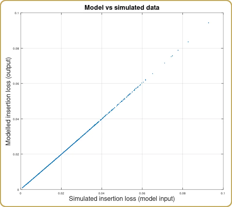
As expected, we got a good correlation between the simulations and the model expansion. Since the physical optics is only described by the overlap integral, that was to be expected. After all, this is supposed to be an example to learn from.
Now, we can also have a look at how much of this correlation comes from the linear term,
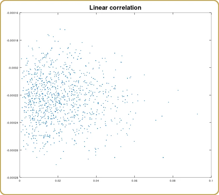
And again, as expected, the correlation is a (statistical) zero. We modelled something that has a minimum at zero aberrations. The linear part is expected to vanish. So now, let’s have a look at the square term.
I hope that by now, it’s pretty obvious that we are going to use the Singular Value Decomposition, remember the red pill, right? So, we throw our H into the SVD, and the first thing to scrutinize are the singular values,
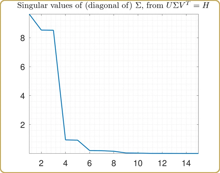
The actual values on the Y-axis are not so interesting, after all, they depend on the volume of our test hypercube, which we used to sample our problem. What’s more interesting is the structure. Our problem has been reduced to almost 3 independent variables, plus 2 much less important ones. Let’s have a look,
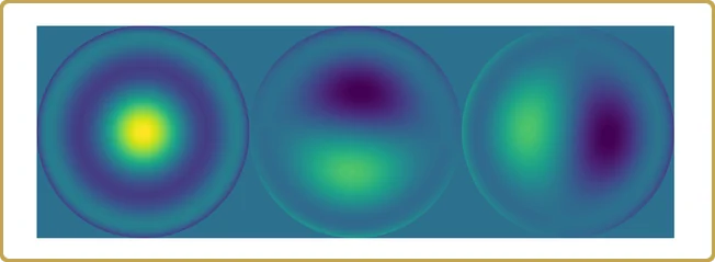
Time to sum up.
We started with 1024 simulated values over 15 dimensions of something we (pretended to) know nothing about, and ended up with 3 major contributions to a property we wanted to understand.
This is not an unusual result when doing this type of analysis. Perhaps the correlation is not quite as good as in this constructed example, but with some transformation of the data, the 2nd order model can capture essentially all the variance of the simulation.
Perhaps the most valuable aspect of this type of analysis is that we can take on a much larger number of degrees of freedom and not restrict ourselves by our ability to untangle the complexity, or to connect to the map metaphor, there are no trees. Woods and hills are all we see. From this vantage point, the big picture is all there is, and all we paid for it was computer time.
Systems engineers toolbox
There is a practical tool in here, for systems engineers who just need a way to capture one of many moving parts in their (usually quite large) Excel sheet of system trade-offs.
It’s not always that one will find a textbook analysis like the one presented here. I’m writing this because I just ran into one where there is no linear correlation, and no second-order correlation, but the full expansion still captures 96%-97% of the data. This is not unusual when one mixes variables that are not physically connected. They usually don’t model well together.
However, the expansion still captured information which can be used when we, as systems engineers, need to trade between parameters that we capture in our (say) optical simulations against the effects these parameters may have on other system properties. Many such examples.
Going further
Why did we stop at a 2nd order expansion? Well, there are “reasons”. The next order is described by a symmetric rank-3 tensor. We can still extract the components of this tensor because the least-squares problem coupling these components to our data is still linear.
There are some things we lose though. There is no SVD for tensors, for example. However, there is “recent” mathematical work done here (if you call 2005 recent, but I started doing this before 2005, so), that may offer further insights into properties of complex systems, such as eigenvalues and eigenvectors for tensors.
If you find that too esoteric, and I completely understand if you do, a 3rd order expansion is guaranteed to capture more variance in your data than a second-order. If you just need that magic function in your Excel sheet, at least you can have that.