


This blog post will be the first of three about the appliation of Goodman’s graphical methods and partially coherent illumination with focus on its application to spatial light modulators. This introduction will start at a point before Goodman’s paper and end just about where his paper begins. Hopefully, it will serve as an introduction to the teminology and concepts in the paper.
Partial Coherence – Nothing to Fear
Designing a partially coherent imaging system, especially one that involves a spatial light modulator, can be a tall order. Spatial light modulators are complex systems by themselves and to make a design from scratch at the mercy of opaque simulation tools is like illuminating a dark room using a laser pointer. Things become pretty clear at the illuminated spot but the whole picture is still lacking.
The problem with partially coherent imaging is that we are no longer able to fall back on familiar concepts like a linear mapping. With incoherent imaging systems, we can sum intensities. For coherent imaging systems, we sum amplitutes but partially coherent imaging systems are linear in the mutual coherence function, which unfortunately offers very little additional insight into the imaging process.
There is however some relief offered by Goodman. No, not Joseph Goodman. I am talkign about Douglas Goodman. Goodman’s paper, “Graphical methods to help understand partially coherent imaging” is a great paper that offers useful insights into the topic and with the help of a two-dimensional graph some non-intuitive, both quantitative and qualitative, results can be understood.
The papper covers the topic from serveral vantage points but jumps into the story assuming that the reader is familjar with the formalism. This, in my experience, is sometimes a bridge too far for many readers. Therefore, this Tech Talk will attempt to bridge the gap and serve as a prequel to the paper. Since this topic is obviously already rigorously covered in serveral standard texts like Born & Wolf or J. Goodman’s Statistical Optics, we will instead go easy of the theoretical details in order to focus on the most important concepts for the special case of imaging a one-dimensional object, a line.
Back to basics
Therefore, let’s start with something most readers may be comfortable with, the computation of the intensity for a coherent image of an object (O) through an optical system characterized with the impulse response (H). The symbols used here are the same as in the paper to ease the jump to the Goodman’s paper for those inclined to do so.
We have only two hurdles to pass to get the big picture that is the goal here, one is why a one-dimensional object requires a two-dimensional integral. This one is simple because it involves expanding the expression above into its amplitude and complex conjugate. Voila. Two integrals. Are we done yet? Well, almost.
How, confession time. There is no such thing as partial coherence. Quantum physics tells us that a particle interferes only with itself or not at all. That’s pretty square, ain’t it? When we set up a partially coherent system, we basically need an incoherent source with sufficient etendue to illuminate all the objects we want to squeeze into a single image. For the topic at hand, we can forget about etendue but we need to consider the incoherent source at infinity, or practically speaking, at the other end of a collimated 2F system.
So, does it mean we can just sum the intensities for all the plane waves originating from the source?
No, it does not because the integral above does not correctly account for the off-axis illumination. Our impulse response (H) does not care about the direction of the light because a point source radiates into the half-sphere whether we illuminate it from the side or head-on. However, to describe the extended object (O), we must account for the varying phase implied by the off-axis illumination. Hence, the basic coherent (per source point) integral must be expanded into,
We now have three integrals instead of the promised two. We take care of tihs by collecting all terms that depend on the incident direction and squeeze all of that into something we will call the mutal coherence function (J),
And finally, lets collect all of the above and we have our final expression for the 1D case of a partially coherent image,
Many details have been ommitted for the sake of not missing the forest for the trees, and the forest in this case is (1), that we have expanded the intensity into an amplitude and its complex conjugate and (2), made an incoherent sum over the intensities in (1). In this process, we managed to isolate a Fourier transform over the distribution of the spectral density (in reciprocal space) of the incoherent source.
When looking at the expression for J(), the electrical engineer might come to think of the Wiener-Khinchin theorem wich relates the Fourier transform of a spectral density to an autocorrelation. In optics, the same piece of math is called The Van Citert-Zernike theorem. The math is the same but the integral is over reciprocal space.
The graphical view
Now that it should be clear why the formalism looks the way it does, It’s about time we make the connection with Goodman’s paper.
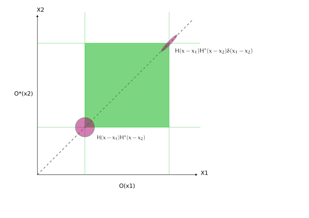
The depicted figure illustrates two distinct imaging cases simultaneously: coherent imaging in the lower left and incoherent imaging in the upper right. Magenta shapes within the graphic attempt to encapsulate the symmetry of the integrand. In Goodman’s paper, this is referred to as the “projector function,” which emerges from the product of the impulse response and the coherence function.
When the light source encompasses a wide solid angle, the coherence function experiences significant cancellation within its integral. Consequently, non-zero values of the coherence function are found primarily near the diagonal. In contrast, for coherent illumination, the coherence function maintains a consistent value across the entire plane. This consistency is symbolized in the figure by a circle, which emphasizes the symmetry properties of the projector function, denoted HH*.
So, what insights can we infer from this visualization? The intensity, I(x), emerges from the convolution of the projector function with the object – represented by a square – along the diagonal where x1 equals x2. A direct observation from this is that, in coherent imaging, the value of I(x) at the object’s edge is a mere quarter of its value within the object’s interior. This implies that for an object to be effectively exposed using coherent illumination, the dose needed for a high-contrast resist is quadruple the dose to clear it.
Conversely, for the incoherent imaging portrayed in the upper right, the correct exposure dose for incoherent imaging is double the dose to clear. This is because half of the projector function resides within the object, while the other half lies outside, as illustrated by the products O(x1)O*(x2).
These interpretations are the most apparent outcomes of Goodman’s graphical method, but there are myriad others, which will be the focal point of upcoming Tech Talks. While the primary applications of this method are rooted in lithography, it occasionally finds relevance in interferometry as well.
Our subsequent blog post will delve into how the imaging properties are influenced by imperfections or intentionally incorporated traits of various spatial light modulators. Stay updated by registering on our contact page.